Wednesday, August 9, 2017
I had mentioned in a previous post that IPM's require both d and q-axis currents for optimal performance. Thanks to the motor equations, it is easy to quantify this split.
Recall that a sinusoidally-varying motor is modeled by:$$ \begin{array}{lcl} \tau=\frac{3}{2}n_p(\lambda I_q+(L_d-L_q)I_d I_q)\\ V_d=R_s I_d-\omega L_q I_q\\ V_q=R_s I_q+\omega L_d I_d+\omega\lambda\\ V_s=\sqrt{V_d^2+V_q^2}\\ I_s=\sqrt{I_d^2+I_q^2} \end{array} $$ Suppose we have unlimited back EMF, and we wish to optimize torque per amp. There are two ways to look at this. Firstly, we could $$ \mbox{minimize } \begin{cases} I_d^2+I_q^2\mbox{ subject to}\\ \lambda I_q+(L_d-L_q)I_d I_q=\tau_0 \end{cases} $$ Or, we could $$ \mbox{maximize } \begin{cases} \lambda I_q+(L_d-L_q)I_d I_q\mbox{ subject to}\\ I_d^2+I_q^2=I_0^2 \end{cases} $$ As it turns out, the second current-first approach results in much easier math (we only need to solve a quadratic, not a quartic) at the expense of being somewhat less intuitive (it is unclear what current corresponds to what torque).
There are several ways to solve the second problem; we use Lagrange multipliers here. The Lagrangian is $$L(I_d,I_q,u)=\lambda I_q+(L_d-L_q)I_d I_q-u(I_d^2+I_q^2-I_0^2)$$ where \(u\), not \(\lambda\), is the multiplier. The system of partial derivatives is $$ \begin{cases} \frac{\partial L}{\partial I_d}=(L_d-L_q)I_q-2I_d u=0\\ \frac{\partial L}{\partial I_q}=(L_d-L_q)I_d-2I_q u+\lambda=0\\ \frac{\partial L}{\partial u}=I_0^2-I_d^2-I_q^2=0 \end{cases} $$ This system is easily solved by a computer algebra system or by multiplying the first equation by \(I_q\) and the second by \(I_d\), giving $$ \begin{array}{lcl} I_d=\frac{-\lambda+\sqrt{\lambda^2+8(L_d-L_q)^2I_0^2}}{4(L_d-L_q)}\\ I_q=\sqrt{I_0^2-I_d^2} \end{array} $$ where we have picked the signs knowing that \(I_d\) is negative and \(I_q\) is positive.
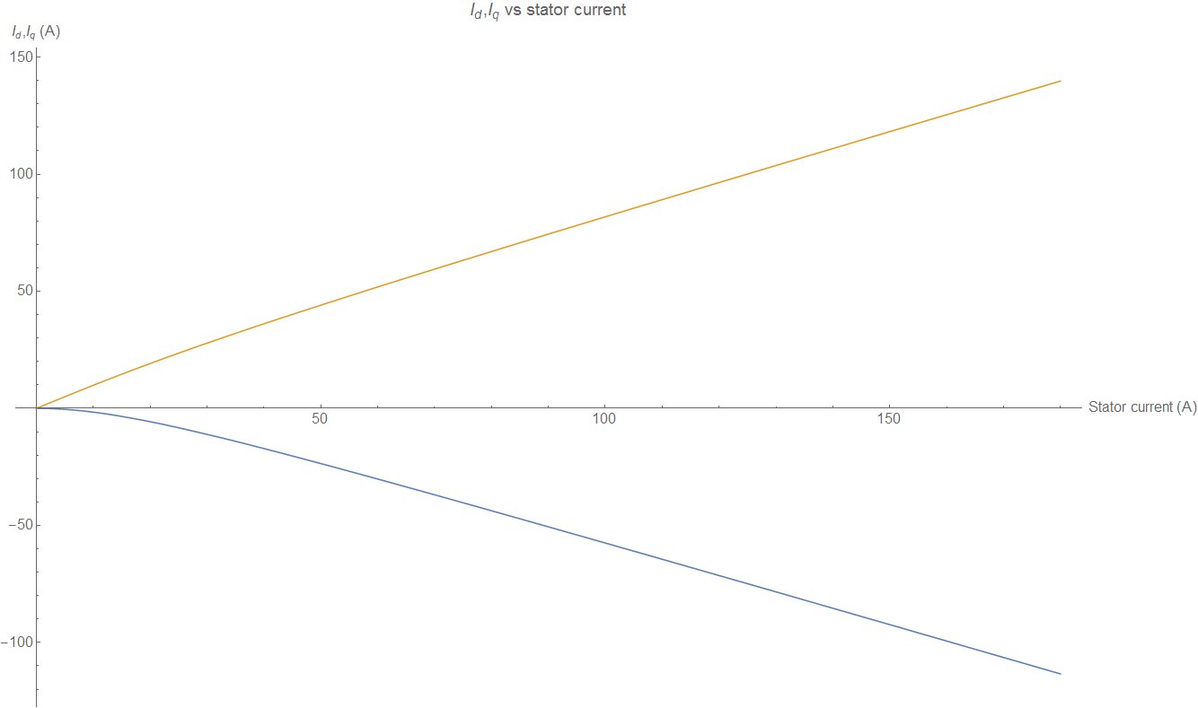
Armed with this information we can make some plots. Plugging in the HSG data \(L_d=0.0006\), \(L_q=0.0015\). and \(\lambda=0.053\) (units: Henries, Volt-seconds), we have the following plot:
As expected, \(I_d\) is about the same magnitude as \(I_q\) at high currents.